Imagine you are asked to write a function to find a median of a given list of numbers. Easy peasy right? And given that the list is unsorted you sort it inside your function.

def calculate_median(nums):
    if len(nums) == 0:
        return 0
    nums = sorted(nums)
    if len(nums) % 2 == 1:
        return nums[len(nums) // 2]
    else:
        return (nums[len(nums) // 2 - 1] + nums[len(nums) // 2]) / 2

But what if the list keeps growing indefinitely, and you need to find the median in real time? This scenario presents a challenging problem known as the "Infinite Rolling Median Problem."

To address this issue, we will progressively enhance simple approaches and gradually develop a solution that, to the best of my knowledge, is the most optimal for this problem.

Naive Approach

Let's keep things simple and assess the capabilities of the naive approach in solving this problem. We will utilise our implemented calculate_median function to test the problem and determine the time and space complexities of the solution.

import random

def calculate_median(nums):
        # ... same as before

def naive_solution(N):
        data = []
        for _ in range(N):
                rn = random.random()
                data.append(rn)
                median = calculate(median)

Assuming that calculate_median which uses Python’s default sorted function and it has an optimal time-complexity of \(O(Nlog(N)\) and that for each in naive_solution, we loop over \(N\) means that the time-complexity would be \(O(N^2log(N))\) which is not that bad for smaller \(N\) but would increase rapidly with larger \(N\).

To understand the execution of the function we will be carrying out multiple runs for each specific \(N\) and calculate the average time taken to execute it.

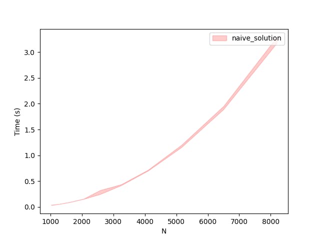
The above graph shows the runtime of 10 runs for each specific \(N\) ranging from 1000 to over 8000. As you can see the runtime increases in close to a power of two.

Sorted List

Upon examining our naive solution, it becomes evident that a more efficient approach would involve maintaining the incoming numbers in a sorted list instead of sorting the list repeatedly within the compute_median function. By doing so, we can reduce the time complexity of the compute_median function to \(O(1)\). Furthermore, this adjustment allows us to keep the list nearly sorted as new numbers are added, resulting in a more efficient sorting operation with time complexity\(O(Nlog(N))\).

def compute_median(nums):
  if len(nums) == 0:
      return 0

  mid_index = len(nums) // 2
  if len(nums) % 2 == 1:
      return nums[mid_index]
  else:
      return (nums[mid_index-1] + nums[mid_index]) / 2

def sorted_list_solution(N=100):
    data = []
    for _ in range(N):
        r_num = random.random()
        data.append(r_num)
        data.sort()
        median = compute_median(data)

We conducted a comparison between our naive_solution and sorted_list_solution by measuring their execution times across a range of numbers. The mean and deviation of the execution times were then plotted for analysis and evaluation.

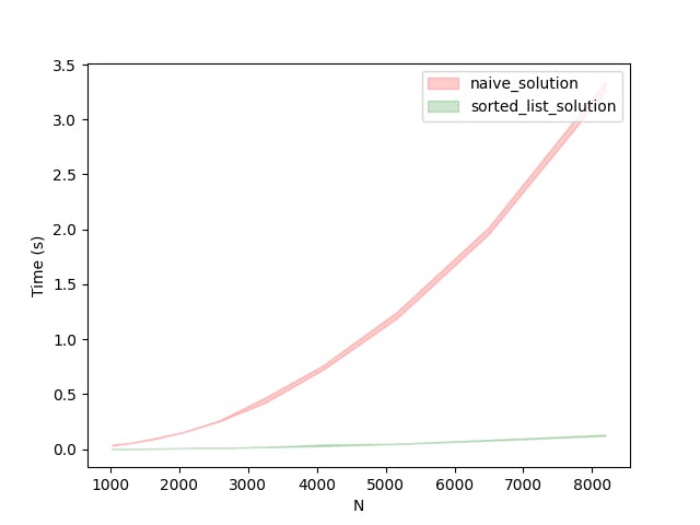
By maintaining the list sorted, as demonstrated in the previous solution, we have achieved a substantial performance boost. However, we are not done yet. We will continue building upon this improved solution to explore further enhancements and push the boundaries of its performance capabilities.

Bisect Package

In the Python standard library, bisect is a package a set of functions which allows for efficient sorting of lists using binary search. A similar solution to that of sorted_list_solution is written below using bisect.

import bisect

def compute_median(nums):
    ## similar to previous

def bisect_solution(N=100):
    data = []

    for _ in range(N):
        r_num = random.random()
        bisect.insort(data, r_num)
        median = compute_median(data)

Since the native_solution takes a lot of time for execution, we will no longer be comparing its runtime with other solutions. We will be focusing only on better solutions going forward.

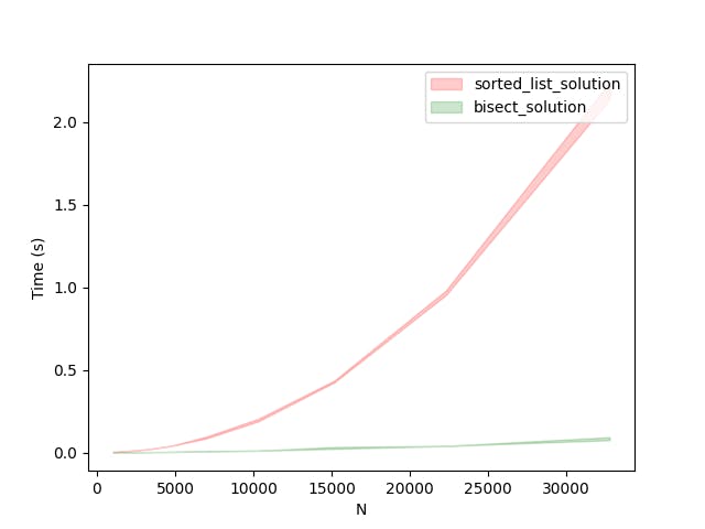
As evident from the above comparison between our sorted list approach and bisect approach, we can immediately see that for much larger N the bisect_solution outperforms the one which just sorts the list.

Tracking the Median

To devise an even more efficient solution, it is crucial to reflect on the ultimate objective we aim to accomplish. Our primary goal is to maintain a continuous track of the median. Consequently, it is worth exploring the possibility of developing a system that not only effectively retains the median but also seamlessly accommodates the insertion of new numbers.

By focusing on this core objective, we can strategise and implement an optimised solution that prioritises the efficient tracking of the median while ensuring that the insertion process remains smooth and seamless. This approach enables us to strike a balance between accuracy and performance, leading to an enhanced system for effectively managing the median and incorporating new numerical values.

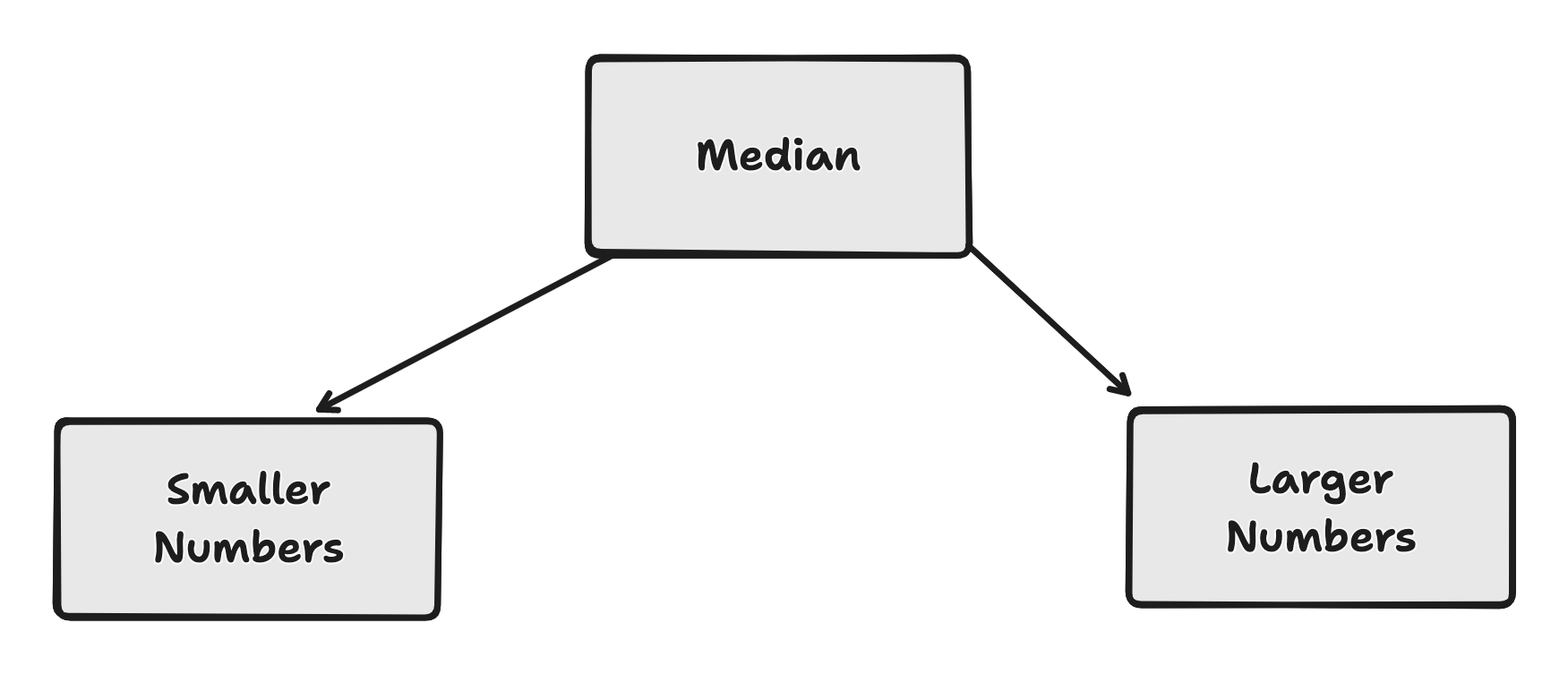
The underlying concept involves efficiently storing the left (smaller values) and right (larger values) sides of the list. The median number will be tracked separately, enabling us to determine the appropriate placement of new numbers. To accomplish this, a heap data structure from the heapq package in the standard Python library has been utilised for its efficiency.

By leveraging the heap data structure, we can ensure efficient insertion and retrieval operations while maintaining the desired order of the values on the left and right sides of the list. This approach facilitates an optimised implementation of the median tracker.

Considering the efficiency of heaps in maintaining the smallest value, we can easily handle the right side (larger numbers) of the median calculation. Retrieving the smallest larger number than the current median requires constant time complexity\(O(1)\), and inserting it into the heap takes \(O(log(N))\) time complexity.

However, dealing with the left side (smaller numbers) is slightly more complex. To retrieve the largest smaller number than the current median, we need to manipulate the values. To facilitate this, we can store the negation of each number (i.e., -x) to simplify the process and make it easier for the heap to find the largest smaller number.

This approach enables us to efficiently handle both sides of the median calculation, maximising performance by leveraging the strengths of heaps while considering the unique requirements of each side.

To implement the median tracker, it is important to establish the requirements that it needs to fulfil. The tracker should be able to:

1. Add a number to the tracker.

2. Retrieve the median from the numbers added so far.

Given that we intend to store the median and maintain separate structures for the right and left sides of the list, the structure of the MedianTracker class would appear as follows.

class MedianTracker:

        def __init__(self):
                self.r_set = [] # larger values
                self.l_set = [] # smaller values
                self.mid = None

        def add_number(self, n):
                ## to be implemented

        def calculate_median(self):
                ## to be implemented

Inserting Numbers to Median Tracker

Maintaining the invariant of the structure during the insertion process is crucial to ensure that we always keep track of the median of the numbers added thus far. This requirement can be simplified into two scenarios: when the current median is less than the incoming number, and when the current median is greater than the incoming number.

To consider a number as the median, we must have a balanced set of numbers on the left and right sides of the median. Therefore, while inserting numbers into the median tracker, it is essential to ensure a well-balanced number of items on both sides of the median. The following code presents an implementation that satisfies these conditions.

class MedianTracker:
        ## ...

        def add_number(self, n):

        if self.mid is None:
            self.mid = n
            return

        # check if the sides are balanced
        # if a number is greater than mid -> take the number and put
        #   it to the right side and take the least of the right side
        # if a number is less or equal to mid -> take the number and put
        #   it ot the left side and take the largest of the left side
        # replace the mid with the largest or the smallest values
        #   from either side
        d = len(self.l_set) - len(self.r_set)
        if d == 0:
            if n > self.mid:
                heapq.heappush(self.r_set, n)
            else:
                heapq.heappush(self.l_set, -n)
        elif d > 0:
            if n > self.mid:
                heapq.heappush(self.r_set, n)
            else:
                largest_l = heapq.heappop(self.l_set)
                heapq.heappush(self.r_set, self.mid)
                self.mid = -largest_l
                heapq.heappush(self.l_set, -n)
        else:
            if n > self.mid:
                smallest_r = heapq.heappop(self.r_set)
                heapq.heappush(self.l_set, -self.mid)
                self.mid = smallest_r
                heapq.heappush(self.r_set, n)
            else:
                heapq.heappush(self.l_set, -n)

        ## ...

The core idea behind the implementation is to consider the disparity between the left and right sides of the median, as well as the appropriate placement of new numbers. By analysing this difference, necessary adjustments can be made to maintain a balanced distribution on both sides.

When the difference between the left and right sides is zero, indicating a balanced state, the process becomes relatively straightforward. If the new number is smaller than the current median, it is added to the left side; if it is greater, it is added to the right side.

However, when the difference is non-zero, an additional operation is required. This operation involves transferring a number from the side with a greater number of elements to the side with fewer elements. This step ensures the continual balance between the two sides, guaranteeing the integrity of the structure.

By employing this approach, we can effectively manage the median tracker while preserving the equilibrium of the left and right sides throughout the insertion process.

Calculating the Median

Calculating the median itself is a relatively straightforward function to implement. First, we need to determine the total number of elements, which is the sum of the elements on the left side, the right side, and an additional 1 for the midpoint itself.

If the total number of elements is odd, we can simply return the current median as the output, as we have a single middle value. However, if the total number of elements is even, we need to take the average of the median and either the largest value on the smaller side or the smallest value on the larger side, depending on which side contains the greater number of elements.

class MedianTracker:
        ## ...
        def calculate_median(self):

        if self.mid is None:
            return 0

        if (len(self.r_set) + len(self.l_set) + 1) % 2 == 1:
            return self.mid

        if len(self.r_set) > len(self.l_set):
            x = self.r_set[0]
            return (x + self.mid) / 2
        else:
            x = -self.l_set[0]
            return (x + self.mid) / 2
        ## ...

Performance Comparison

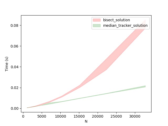
In terms of time complexity, the MedianTracker solution offers an improvement. The insertion of numbers in the MedianTracker takes a maximum of O(log n) time complexity due to the balancing operations performed, ensuring that both sides of the median remain relatively equal. On the other hand, the calculation of the median in the MedianTracker solution has a constant time complexity of O(1), as it directly retrieves the median value based on the maintained structure. From the graph below it is evident that the MedianTracker solution is outperforming the bisect solution.

Comparing Solution

Below is a graph comparing the performance of the most efficient approaches we have implemented thus far. As depicted in the graph, the MedianTracker solution and the bisect solution are compared. It is evident that for smaller values of N, the performance of the MedianTracker solution is comparable to that of the bisect solution. However, as N becomes larger, the MedianTracker solution starts to outperform the bisect solution significantly. This indicates that the MedianTracker solution excels in handling larger datasets and provides better scalability.

Conclusion

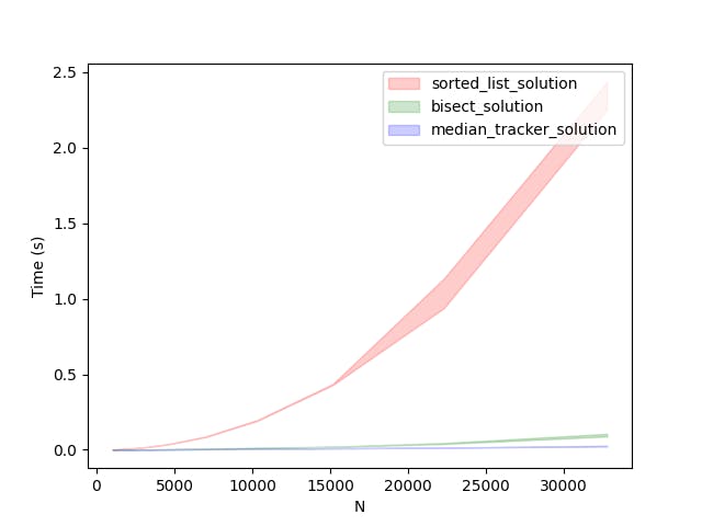
Among the three approaches - the sorted list solution, bisect solution, and median tracker solution - for calculating and tracking the median in a growing list of numbers, the median tracker solution stands out as the most optimal. While the sorted list solution suffers from repeated sorting operations and has a time complexity of \(O(N^2log(N))\), and the bisect solution improves upon it with a time complexity of \(O(Nlog(N))\), the median tracker solution outperforms both by maintaining the balance of the left and right sides. With a time complexity for each insertion and \(O(1)\) for median calculation, the median tracker solution offers efficient real-time tracking of the median. It also provides better scalability and performance as the number of elements increases. Moreover, the space complexity remains \(O(N)\) for all three solutions. Therefore, the median tracker solution emerges as the most efficient and optimal approach for solving the "Infinite Rolling Median Problem."

Source Code: https://github.com/THasthika/rolling-median